Introduction

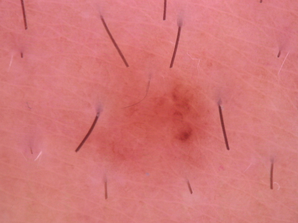
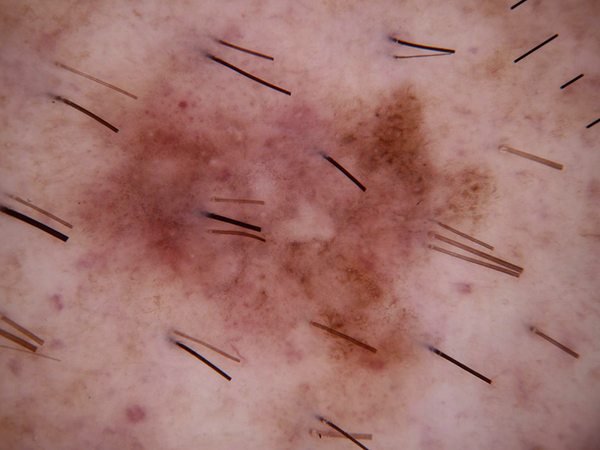
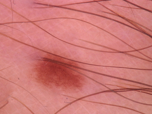
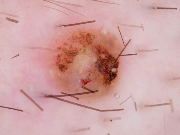
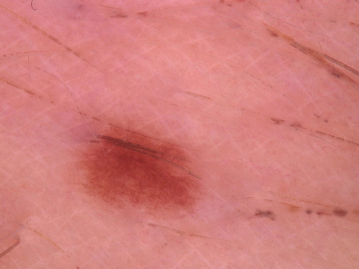
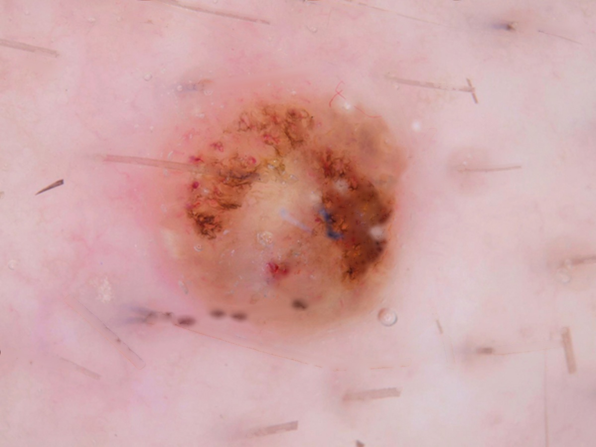
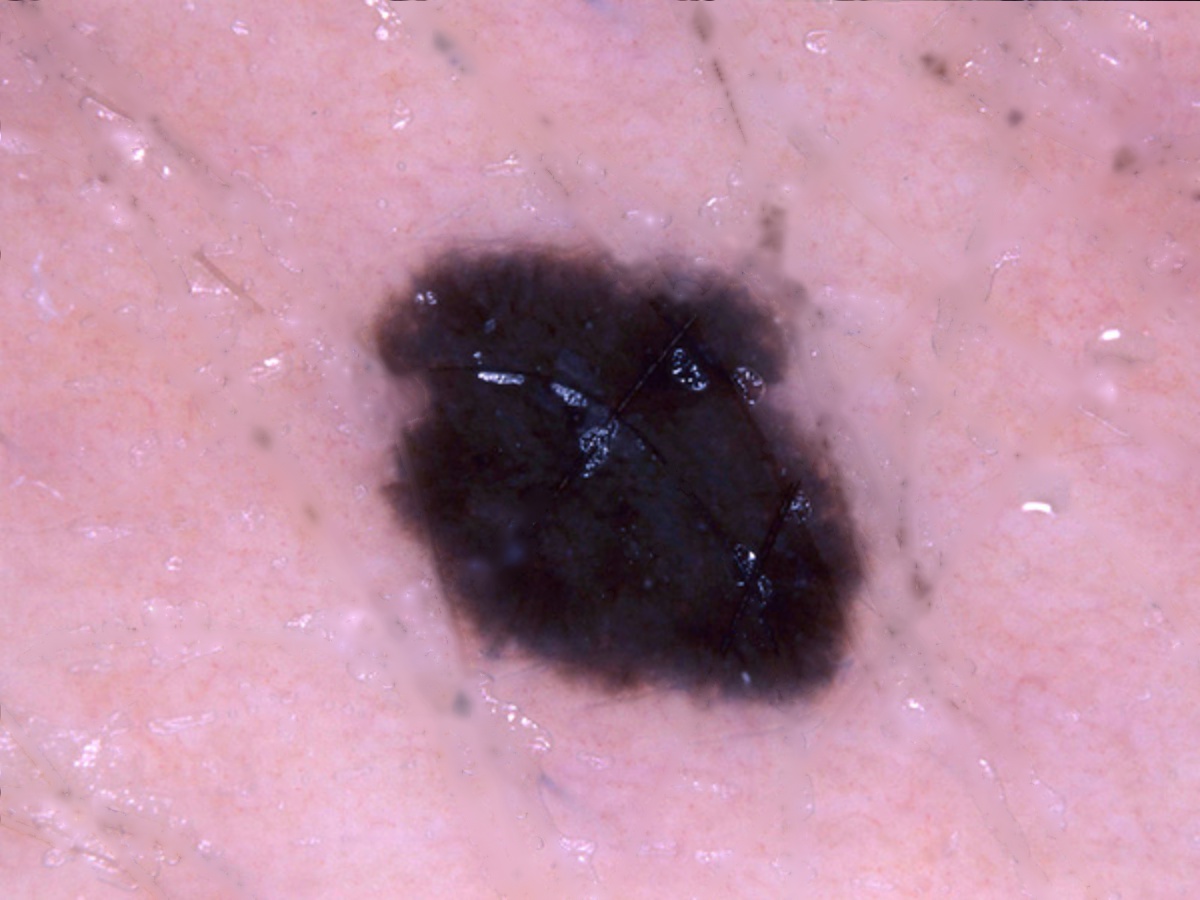
Skin cancer has become a commonly encountered disease in recent years. To improve the skin cancer detection accuracy and enhance the associated disease treatment, International Skin Imaging Collaboration (ISIC) held this challenge and provide a large and publicly available image dataset collection for skin cancer research.

Image pre-processing

The dermoscopic images usually contain hairs, which can be considered as noises that may degrade the model prediction accurate. Before the model training and, preprocessing the images to remove the hair regions may be helpful to the model prediction accuracy. In this work, we propose to preprocess the dermoscopic images to remove hairs in the images. By using adaptive thresholding to obtain relatively darker and lighter areas in the input image, we can filter out hair and scars from other parts. Then we separate hairs from scar based on the different characteristics in the image appearance and replace hair regions with blurred images. Last, we apply the color constancy [1] for each image.

Three Tasks

Lesion Segmentation

To provide automated predictions of lesion segmentation boundaries from dermoscopic images.

Lesion Attribute Detection

To automatically predict the locations of dermoscopic attributes from dermoscopic images. The classes include: pigment network, negative network, streaks, milia-like cysts, globules (including dots).

Disease Classification

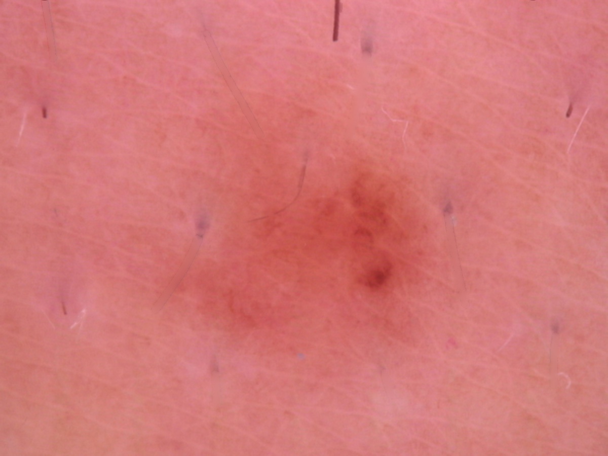
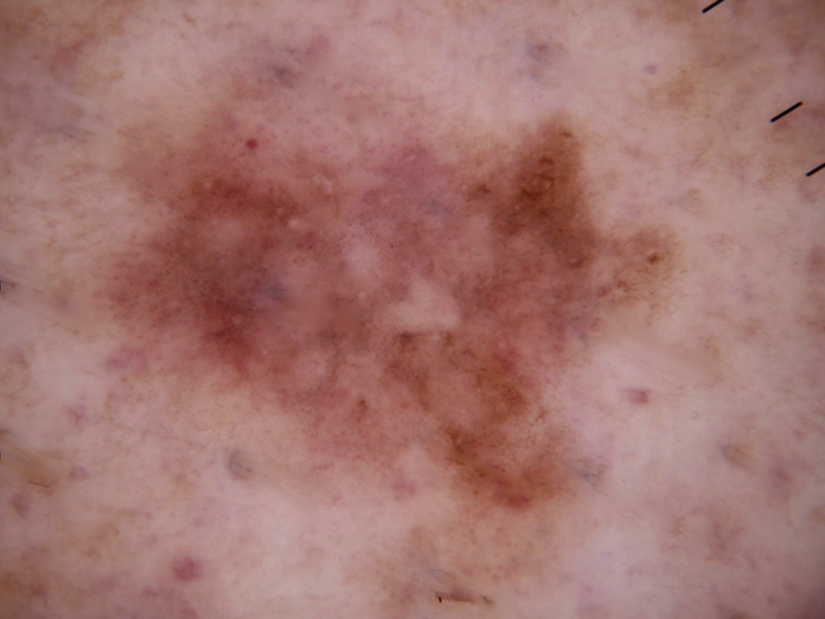
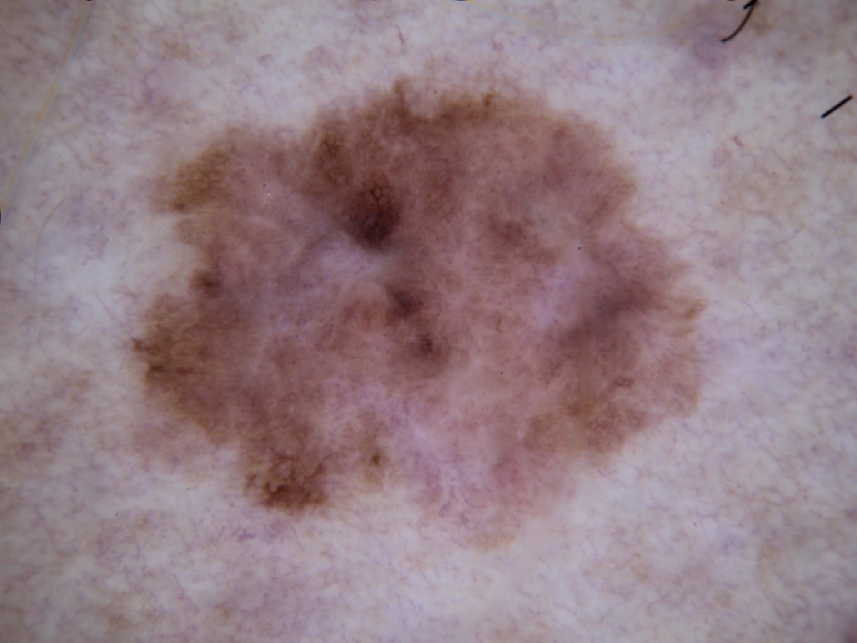
To classify disease category from dermoscopic images. The classes include: Melanoma, Melanocytic nevus, Basal cell carcinoma, Actinic keratosis / Bowen’s disease, Benign keratosis, Dermatofibroma, Vascular lesion.

We propose to train convolutional neural network (CNN) models for each of the three tasks with the training datasets provided by in the challenge. The details of the model training and model validation results are described in the subsequent sections.

Image Pre-processing

By observing the dermoscopic images, we found out the characteristic of hair noises include: they normally looks slender and not circle, and they normally is darker than surrounding skin. So my detection method is based on these two points.

Adaptive Thresholding

 First, I found out the areas which are relatively darker than neighbors by adaptive thresholding. Adaptive thresholding is an extend in thresholding: in normal thresholding, the reference threshold is based on the mean of whole range; in adaptive thresholding, the threshold for each point is the mean calculated based on the neighbor area. The advantage of adaptive thresholding includes dynamic block size and threshold offset.

Geometric Shape

 After filtered out all the related-darker area, the next step is to pick out the hair area in these contours. Under the first selection, hair, scar and stage micrometer will be collected. Hair and stage micrometer are noise to a disease image, so both of them are chosen to remove from images. There are some difference in the two group of characteristic which I want to separate: for hair and stage micrometer, they usually look slender; for scar, it usually has a hollowed look and might cross large area. I will separate them based on their geometric shape. I used 2 methods to calculated their difference:

1. Ratio between radius of external circle(r) and perimeter(s):

  • s/r = 2𝜋 : this contour is circle.
  • s/r ≈ 4 : this contour might be a straight line crossing the center of external circle.
  • s/r becomes larger : this contour might be a curly, spiral line or multi-hollowed shape.

2. Ratio between area(A) and area of external circle(A’):

  • A/A’ larger : the contour is close to circle or concentrated net structure.
  • A/A’ smaller : the contour is more close to a slender line or loose net structure.

Remove and fill-in hair area

After getting mask the original image, I removed the noises from origin image, then used the inpaint function to fill-in the hair(noise) area, and recovered the image without hair.

Before in-painting, to make sure all noises including the edges of noise are all included, I first dilate the mask to ensure edges won’t become the sample for in-painting. I used the inpaint function in opencv to recover images. This function is designed based Telea’s FMM inpaint method.

 The main principle of Telea’s FMM is in Fig 1. and below formulas. Every recovery work starts from a point p in the set of boundary. First, pick the p that has the largest sampling area(the area with radius epsilon.) The final value of point p is the sum of every sampling points with weighting w(p, q).

 The weighting is based on three geometric factors: direction relationship, distance relationship, and level relationship. Direction relationship is calculating the distance between normal vector and sampling point q: if q is close to normal vector, it gets higher weight; vice versa. Distance relationship is depends on the distance between p and q: if they’re closer, it gains higher weight, vice versa. Last but not least, level relationship is based on the contour: if q is closer to contour, it earns higher weight; vise versa.


Lesion Segmentation

The goal of task 1 is to predict the boundary of skin lesion from dermoscopic images. Each image contains only a single contiguous region. The goal metric is computed using a threshold Jaccard index. The final score is taking the mean Jaccard index of each image but images with scores less than 0.65 are count as 0.

Dataset

 The ISIC 2018 Challenge provides 2594 dermoscopic images with various sizes for task1 and task2. We divide the images into 2494 training data and 100 validation data. The preprocessing described is first applied to get rid of the hair and other obstacles. The images are then resized to a fixed size of 256 × 256.

Model Architecture and Training

We use the global convolutional network (GCN) and the same pipeline described in [2]. GCN uses a combination of 1 × k + k × 1 and k × 1 + 1 × k convolution, which can have a better receptive filed without increasing the number of parameters dramatically. Since the goal of this task is to identify the boundary, larger receptive filed can give the model more global information and thus performs better. The kernel size parameter k of the model is set to 7 and the dimension is reduced to 1 to match the number of classes of the dataset. Sigmoid nonlinearity is applied at the output.

Since the challenge uses Jaccard index as the goal metric, we use Jaccard loss similar to as our loss function.

where yij ∈ [0, 1] and tij ∈{0, 1} are the output and target for each pixel at position (i, j).

 Data argumentation of random horizontal flip and vertical flip are used. The model is trained via Stochastic Gradient Descent (SGD) optimizer with the learning rate set to 0.001 and drop the learning rate by a factor of 0.1 once the loss reaches plateau twice. The batch size is set to 6 and the network is trained about 100 epochs.

Lesion Attribute Detection

In task2, we need to identify 5 kinds of dermoscopic attributes: pigment network, negative network, streaks, milia-like cysts, and globules. We use one binary mask for each type. The goal metric is Jaccard index.

Dataset

 We separate the 2594 images into training and validation data as described in task1. The images are resized to 512x512 without preprocessing. Other than the 5 given classes, we add a no-finding class. That is, when a pixel does not belong to any of the 5 classes, it belongs to the no-finding class as depicted in Figure 1. By adding the no-finding class, we can compute softmax directly from the output.

Model Architecture and Training

The same GCN [2] model is used with kernel size k = 7. The dimension is set to 6 to match the 5 classes and the no-fining class. Softmax is applied at the output.

The difficulty we encountered for this task is that the data is highly unbalanced. Most images have no positive instances for the attributes except the pigment network. As the result, we tried different loss functions. We found that a combination of weighted cross entropy loss and Jaccard loss works the best. The weighted cross entropy loss is given as follows:

 The model is trained via Stochastic Gradient Descent (SGD) optimizer with the learning rate of 0.0001. The batch size is 6 and the model is trained about 80 epochs.

Lesion Diagnosis

The goal of Task 3 is to generate predictions from dermoscopic images for the following 7 disease categories: Melanoma (MEL), Melanocytic nevus (NV), Basal cell carcinoma (BCC), Actinic keratosis (AKIEC), Benign keratosis (BKL), Dermatofibroma (DF), Vascular lesion (VASC). The response data should include diagnosis confidence, which lies in a closed interval [0.0, 1.0], for each class. The evaluation is computed using a normalized multi-class accuracy metric.

Dataset

 In Task 3: The official provides 10015 images and 1 ground truth response CSV file. The numbers of images for each class are: 1113 for MEL, 6705 for NV, 514 for BCC, 327 for AKIEC, 1099 for BKL, 115 for DF, 142 for VASC . We divide this dataset into 8012 training samples and 2004 validation samples. The ratio for training data to validation data is approximately 4:1. The images are preprocessed to eliminate the hair and leave us more clear lesions. Then the images are resized to 224x224.

Class MEL NV BCC AKIEC BKL DF VASC
# images 1113 6705 514 327 1099 115 142

Model Architecture and Training

 We use ResNet-50 [4] as our training model. ResNet introduces the concept of Residual function to solve the problem that using deeper networks will degrade the performance of the model. It uses kernel size of 1 or 3 and down samples with CNN layers of stride 2. We add our fully-connected layer at the end of the network to classify 7 classes as needed. Using Softmax to calculate the probability for each class. Cross entropy is used as our loss function.

where x is the output of the model and class is the index of ground truth class.

 We use SGD as our optimizer with a learning rate of 0.001 The batch size is set to 8 and trained about 300 epochs.

Result -- Image Pre-processing

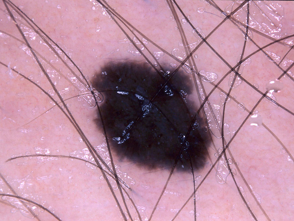
 In the below table, we show part of the results after image pre-processing.

Before Image Pre-processing
After Image Pre-processing

 The above images are part of the results. Repairing results are not that good in two situation: lots of hair gathered or crossed together, and hair too light.

 About the first point: when the dark area is larger than the block size adaptive thresholding, the center of the hair won’t be picked out. When repairing with in paint method, the center of the hair will become the sampling area to in-paint the removed area, and cause the repairing mistakes.

 Second, some transparent hair won’t be detected via this detecting method. To avoid this situation and remain the scars and important points are quite difficult by detecting only intensity. But I haven’t found a better solution for keeping both of them at this time. This can be my future work.

Result -- 3 tasks

 The scores of all 3 tasks are shown in Table 1. For task 1 and task 2, the scores were calculated after applying a threshold of 0.5.

Task Type Task 1 Task 2 task 3
score 0.727 0.379 0.699

Lesion Segmentation

 Most of the models can identify the boundary of the lesion. However, in some cases it may fail to identify the whole lesion and instead only recognize some part of it.

Lesion Attribute Detection

 For task 2, only the pigment network attribute may be poorly identified and other attributes mostly cannot have positive outputs. This is due to the fact that the data is highly imbalanced and we are not able to train the model reliably using the data given.

Lesion Diagnosis

 In task 3, the AUC of our best result is shown in table below.

MEL NV BCC AKIEC BKL DF VASC
AUC 0.700 0.795 0.930 0.936 0.778 0.949 0.917
Final AUC 0.8579

Reference

[1] Catarina Barata, M. Emre Celebi, Senior Member, IEEE, and Jorge S. Marques, Improving Dermoscopy Image Classification Using Color Constancy

[2] C. Peng, X. Zhang, G. Yu, G. Luo, and J. Sun. Large kernel matters–improve semantic segmentation by global convolutional network. arXiv:1703.02719, 2017.

[3] Yading Yuan. Automatic skin lesion segmentation with fully convolutional-deconvolutional networks. arXiv:1703.05165

[4] Kaiming He, Xiangyu Zhang, Shaoqing Ren, Jian Sun. Deep Residual Learning for Image Recognition. arXiv:1512.03385, 2015